Qiushi PapersTested on History
How Large Is the Effect of Partner-Currency Volatility on China's Exports? A Re-examination Using Monthly Partner-Level Data, 2000–2025
LuluH. (2026). How Large Is the Effect of Partner-Currency Volatility on China's Exports? A Re-examination Using Monthly Partner-Level Data, 2000–2025 [Working paper]. Qiushi Papers. https://qiushi.luluh.top/en/export-volatility-working-paper/
LuluH. 2026. “How Large Is the Effect of Partner-Currency Volatility on China's Exports? A Re-examination Using Monthly Partner-Level Data, 2000–2025.” Working paper, Qiushi Papers, November 11, 2026. https://qiushi.luluh.top/en/export-volatility-working-paper/.
@article{luluh2026exporten,
  author       = {LuluH},
  title        = {How Large Is the Effect of Partner-Currency Volatility on China's Exports? A Re-examination Using Monthly Partner-Level Data, 2000–2025},
  journal      = {Qiushi Papers},
  year         = {2026},
  month        = {11},
  note         = {Working paper, not peer reviewed},
  url          = {https://qiushi.luluh.top/en/export-volatility-working-paper/},
  urldate      = {2026-11-21},
  keywords     = {exchange rate volatility, exports, emerging economies, dominant currency pricing, inference with few clusters},
  language     = {english},
}
Export to a reference manager: RIS (EndNote, Zotero, Mendeley) · BibTeX
Cite as: LuluH. (2026). How Large Is the Effect of Partner-Currency Volatility on China's Exports? A Re-examination Using Monthly Partner-Level Data, 2000–2025 [Working paper]. Qiushi Papers. https://qiushi.luluh.top/en/export-volatility-working-paper/
License: Published under CC BY 4.0. You may share and adapt it with attribution. GitHub: github.com/bearkid6/export-volatility
This is a working paper (November 2026 draft). It has not been peer reviewed. This English edition is a translation of the Chinese original (中文版); if the two differ, the Chinese version prevails.
Revised 21 November 2026: the text now states that effects are scaled by the residual standard deviation; a significant robustness check (Table 6, Panel F) is discussed; the limits of the pre-specification claim are stated; references to an online appendix that does not yet exist are removed; Figures 2 and 3 are renumbered; and some bibliographic details and explanatory notes are added. The estimates and the numbers in the tables are unchanged.
Abstract: China’s exports increasingly go to emerging economies with volatile currencies. Whether partner-currency exchange rate risk depresses these exports is still unsettled: most of the existing studies we have found use samples that end before 2016, and few account for the fact that the independent variation comes from only a few dozen currencies. Using monthly exports from China to 96 trading partners and daily exchange rates of 69 currencies over 2000–2025, this paper re-examines the question with Poisson pseudo-maximum likelihood and inference methods suited to few clusters. First, the effect of partner-currency volatility on China’s exports is insignificant both before and after 2010; the confidence sets rule out changes in exports larger than about 1.3% from a persistent rise in volatility of one residual standard deviation (net of fixed effects), or about 2.6% for a rise from the sample median to the 90th percentile, whereas in the same specification a 1% depreciation of the RMB against the partner currency significantly raises exports by about 0.26% within six months. Second, there is no evidence that the effect is concentrated in periods of large partner-currency depreciation. Third, within the same partner and month, partners’ imports from China and from other sources do not respond differently to the volatility of their currency, and the difference is no larger than about 0.5% when scaled by the residual standard deviation in the importer sample. Fourth, product-level data on Hong Kong re-exports and China’s re-imports show no arbitrage-driven round-tripping trade that moves with the China–US interest rate differential, including after the differential turned negative in 2022. A secondary analysis suggests that, relative to other manufacturing exporters, China’s exports to emerging economies fall more when their currencies depreciate sharply, but this result does not survive multiple-testing correction. The results indicate that, at the bilateral aggregate level, everyday partner-currency volatility is not an important determinant of China’s exports, and the exchange rate level deserves more attention.
Keywords: exchange rate volatility; exports; emerging economies; dominant currency pricing; inference with few clusters
JEL codes: F14; F31
1. Introduction
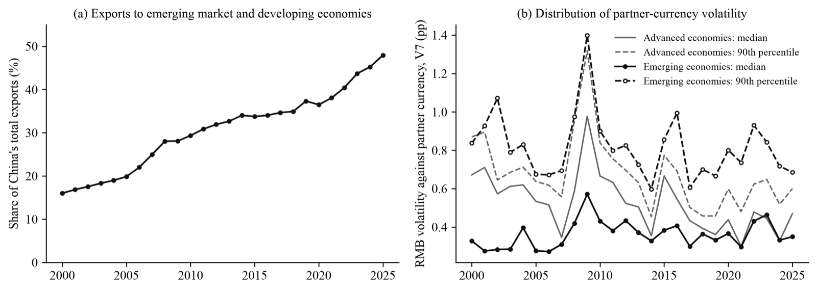
Over the past two decades and more, the market structure of China’s exports has changed markedly. The share of emerging market and developing economies (EMDEs) in China’s exports was 16.0% in 2000, 29.4% in 2010, and 34.9% in 2018, and rose to 47.9% in 2025 (Figure 1a). The currencies of these economies have different risk characteristics from those of advanced economies. Over the sample period, the volatility of emerging-economy currencies against the RMB was not larger in normal times (median 0.36, versus 0.50 for advanced economies; Figure 1b), but their tails were fatter: 3.6% of their months fell in a large-depreciation window, compared with only 0.5% for advanced economies. As export markets shift toward these economies, partner-currency exchange rate risk has become a concern for firms and policymakers: is it already depressing China’s exports, and by how much?
Existing studies do not give a consistent answer. In cross-country studies, the effect of exchange rate volatility on trade varies in sign across samples and methods and is generally small (McKenzie, 1999; Bahmani-Oskooee and Hegerty, 2007; Tenreyro, 2007). Firm-level studies of China find significant negative effects (Héricourt and Poncet, 2015; Tan et al., 2016; Wang et al., 2023), but three issues make these findings hard to apply directly today. First, in the studies of this kind that we have found, most samples end before 2016 and do not cover the period in which export markets shifted rapidly toward emerging economies. Second, the estimated coefficients are not large once converted into economic magnitudes. Statistical significance comes mainly from millions of firm-level observations, while the independent variation that identifies exchange rate volatility comes from only a few dozen currencies, so standard errors clustered by firm or region may understate the uncertainty (MacKinnon and Webb, 2017; MacKinnon et al., 2023). Third, with China’s export data alone, one cannot tell whether the effect comes from the importer side (a partner-currency depreciation depresses the partner’s imports from all suppliers) or from the side of Chinese exporters (settlement currency, trade credit terms, and hedging instruments), and the two have different policy implications (Gopinath et al., 2020).
Using monthly exports from China to 96 trading partners and daily exchange rates of 69 currencies over January 2000–December 2025, this paper re-examines the effect of partner-currency volatility on China’s exports and answers three further questions: whether this effect differs before and after 2010; whether it is concentrated in periods of large partner-currency depreciation; and whether, within the same partner and month, the partner’s imports from China are more sensitive to the volatility of its currency than its imports from other sources. Estimation uses Poisson pseudo-maximum likelihood. Partner × year and year-month fixed effects absorb annual changes in partner demand and the common movements of the RMB against the US dollar, so identification comes from the idiosyncratic volatility of partner currencies against the US dollar. Because independent variation is limited, this paper reports standard errors clustered by currency, jackknife standard errors, and the wild score bootstrap, and bases inference on the last. The specifications, samples, and interpretation rules of the four primary tests were pre-specified before estimation, and the results are reported whether or not they are significant.
There are four main findings. First, the effect of partner-currency volatility on China’s exports is insignificant in both periods, with point estimates close to zero. The confidence sets show that, for a persistent rise in volatility of one residual standard deviation, the change in exports is no larger than about 0.9% over January 2000–June 2010 and no larger than about 1.3% in the full sample. The effects reported in the earlier literature, converted to the same scale, all lie within this range; what this paper can rule out are effects about three times as large as the largest of them. In the same specification, the cumulative elasticity with respect to the exchange rate level is 0.26 and significant, which shows that the insignificant result is not an artifact of the specification or the inference method. Second, there is no evidence that the effect is concentrated in periods of large depreciation. Third, the difference between China and other suppliers is small, no larger than about 0.5%. Fourth, arbitrage-driven round-tripping trade that may be mixed into export statistics does not provide an explanation either: product-level data on Hong Kong re-exports and China’s re-imports show no round-tripping of goods with high value-to-weight ratios that moves with the China–US interest rate differential, and the same holds after the differential turned negative in 2022. The secondary analysis yields one lead: relative to other manufacturing exporters, China’s exports to emerging economies fall more when their currencies depreciate sharply, by about 0.4%–0.5%. This result does not survive multiple-testing correction, and this paper treats it only as a direction for future research.
This paper makes three possible contributions. First, it extends the test of the relationship between China’s bilateral exchange rate volatility and exports to 2025 and uses confidence sets to show how large an effect the data can rule out, so that the insignificant results are informative. Second, using partner-reported import data, it compares China with other suppliers within the same partner and month. This removes partner demand shocks, the main source of endogeneity, and on this basis distinguishes the importer-side channel from the exporter-side channel. Third, on the methodological side, it shows that in this kind of study the effective number of clusters is far smaller than the nominal number of currencies or partners, and that cluster-based standard errors overstate significance. In simulations with synthetic data, standard errors clustered by currency reject the true value at the 5% nominal level in 6.0%–12.5% of cases; in the Hong Kong re-export data, 14 of 29 placebo destinations unrelated to arbitrage obtain “significant” coefficients.
The object of estimation needs to be stated at the outset. Common movements of the RMB against the US dollar are absorbed by year-month fixed effects. This paper answers the question “when a partner’s currency is more turbulent than those of other partners, do China’s exports to that partner fall in relative terms?” It does not address the effect of the volatility of the RMB exchange rate itself on aggregate exports. For the latter, aggregate time series contain only one volatility series, and the data in this paper cannot speak to it.
The rest of the paper is organized as follows. Section 2 reviews the literature and states the hypotheses. Section 3 describes the data, variables, and models. Section 4 reports the baseline results. Section 5 discusses endogeneity and robustness. Section 6 analyzes mechanisms and heterogeneity. Section 7 concludes.
2. Literature Review and Hypotheses
2.1 Exchange Rate Volatility and Trade: Theory and Cross-Country Evidence
The classic explanation for why exchange rate volatility depresses trade rests on risk aversion: in the absence of forward markets, exchange rate uncertainty raises the variance of export revenue, and risk-averse exporters reduce exports (Clark, 1973); the existence of a forward exchange market weakens this effect (Ethier, 1973). Theory does not give a unique answer, however. De Grauwe (1988) points out that higher risk has both a substitution effect, which leads firms to exit, and an income effect, which leads them to export more to make up for the fall in expected revenue; the sign of the net effect depends on the degree of risk aversion. The empirical work is equally inconclusive. The surveys by McKenzie (1999) and by Bahmani-Oskooee and Hegerty (2007) both conclude that the effect of exchange rate volatility on trade varies in sign across samples and methods and is generally small. Rose (2000) finds in a gravity model that bilateral exchange rate volatility significantly reduces trade; Klein and Shambaugh (2006) find that fixed exchange rate arrangements with a direct peg substantially increase bilateral trade. Other studies question the causal relationship. Tenreyro (2007) uses Poisson pseudo-maximum likelihood (PPML) to deal with zero trade and heteroskedasticity, together with instrumental variables, and finds no significant effect of nominal exchange rate volatility on trade. Broda and Romalis (2011) point out that trade itself lowers bilateral exchange rate volatility; once this reverse causality is taken into account, the depressing effect of volatility on trade is small. By sector, Byrne et al. (2008), using sectoral data on bilateral US exports and imports, find that exchange rate volatility significantly depresses trade in all sectors, most strongly for exports of differentiated goods. For emerging economies, Chit et al. (2010) find that exchange rate volatility significantly depresses the exports of five emerging East Asian economies.
2.2 Evidence for China
Earlier studies in China mostly used aggregate or partner-level time series and measured the trade effects of RMB exchange rate volatility with cointegration, error-correction, and GARCH-type models; their conclusions are mixed (Chen and Xiong, 2002; Li and Voon, 2004; Pan, 2007; Gu and Gao, 2007). Later research turned to firm-level customs data. Using firm–destination data for 2000–2006, Héricourt and Poncet (2015) find that firms export less to destinations with more volatile exchange rates, and that financially constrained firms are more affected. Using firm–product–destination data for 2002–2009, Tan et al. (2016) find that bilateral exchange rate volatility reduces export values and the number of products exported, and that the effect is weaker in regions with a higher degree of financial marketization. Xu and Yu (2016) find that better external financing conditions dampen the shock of exchange rate volatility to exports. Wang et al. (2023) find that exchange rate volatility lowers exports and increases exit, and that imports of intermediate goods can offset part of the negative effect. Wang et al. (2016) point out that third-country exchange rate volatility also affects China’s bilateral exports. On the exchange rate level, Li et al. (2015) estimate with firm-level data that the export volume elasticity with respect to the RMB exchange rate is modest; Cao et al. (2016), using data on China and countries along the Belt and Road, find that RMB depreciation helps exports, but only by a small amount; Peng and Liu (2021) re-measure the exchange rate elasticity of bilateral exports from a global value chain perspective; and Thorbecke et al. (2025) find that the exchange rate elasticity of China’s exports fell markedly after the global financial crisis.
These studies share two features. First, the studies we have found that use bilateral exchange rate volatility mostly have samples ending before 2016, whereas the share of China’s exports going to emerging market and developing economies rose faster precisely after that. Second, firm-level estimates obtain statistical significance from millions of observations, but the economic magnitudes implied by the coefficients are not large (Section 4 gives the conversion). Moreover, the independent variation that identifies exchange rate volatility comes from only a few dozen currencies, so standard errors clustered by firm or province may understate the uncertainty.
2.3 Invoicing Currency and the Importer-Side Channel
Dominant currency pricing theory provides a framework for understanding how partner-currency volatility is transmitted. Most global trade is invoiced in a few currencies such as the US dollar (Gopinath et al., 2020; Boz et al., 2022), and China’s exports are also invoiced mainly in US dollars. Under dollar invoicing, a movement of the partner currency against the US dollar first changes the local-currency prices and financing conditions that importers face, and so affects their demand for all dollar-invoiced imports. This is the importer-side channel, and it is broadly the same for all suppliers. Partner-currency volatility may also work through an exporter-side channel. The part of exports settled in the partner currency or in RMB is directly exposed to exchange risk. When the currency is turbulent, the risk that importers delay payment or default rises, and exporters tighten trade credit terms and cut shipments. The fewer hedging instruments, the less trade finance, and the less export credit insurance exporters have access to, the more pronounced this contraction may be (Lu et al., 2019). Whether hedging instruments weaken the effect of volatility is, however, unsettled: Wei (1999) tests this common explanation with data on more than 1,000 country pairs and finds no evidence to support it. This channel differs across suppliers. Distinguishing the two channels matters in practice. If the effect works mainly on the importer side, Chinese exporters are in the same position as their competitors, and there is little they can do. If China’s exports respond more strongly to partner-currency volatility than those of other suppliers, there are links on the exporter side that can be improved. Existing studies use only China’s export data and cannot make this distinction.
2.4 Normal Volatility and Currency Crises
Exchange rate risk in emerging economies differs from that in advanced economies. Many emerging economies operate pegs or managed floats; volatility is low in normal times, and the risk shows up mainly as occasional large depreciations (Frankel and Rose, 1996; Ilzetzki et al., 2019). During currency crises, importers face, in addition to exchange rate uncertainty itself, foreign exchange shortages, import controls, and contracting domestic demand. If the negative relationship between exchange rate volatility and exports comes mainly from these periods, it reflects mostly the shock of crises to import demand, and its policy implications differ from those of “helping firms manage everyday exchange rate risk.”
2.5 Methodological Literature
Two points in the recent methodological literature bear directly on this paper. First, an “insignificant” result is informative only when it is clear how large an effect can be ruled out; confidence intervals and equivalence tests are the appropriate way to present null results (Rainey, 2014; Hartman and Hidalgo, 2018). Second, when clusters are few and differ greatly in influence, cluster-robust standard errors understate uncertainty, and the jackknife and the wild bootstrap are more reliable (MacKinnon and Webb, 2017; Canay et al., 2021; MacKinnon et al., 2023). Studies of bilateral exchange rate volatility fall squarely into this situation: partners using the same currency share one volatility series, independent variation comes from only a few dozen currencies, and a few currencies are far more volatile than the rest.
2.6 Hypotheses
Based on the literature above, this paper proposes four hypotheses.
Hypothesis 1: A rise in partner-currency exchange rate volatility depresses China’s exports to that partner.
Hypothesis 2: With the development of hedging instruments, cross-border RMB trade settlement, and direct trading between the RMB and foreign currencies, this depressing effect has weakened, and it is weaker from the second half of 2010 onward than before.
Hypothesis 3: The depressing effect occurs mainly in periods of large partner-currency depreciation; the effect of normal volatility is smaller.
Hypothesis 4: When partner-currency volatility rises, the partner’s imports from China fall relative to its imports from other sources; that is, a channel on the side of Chinese exporters exists.
All four hypotheses are tested with two-sided tests. If Hypothesis 4 fails but Hypothesis 1 holds, the effect works mainly on the importer side. If both fail, the effect of partner-currency volatility cannot be detected at the bilateral level, and it is then necessary to state how large an effect the data can rule out.
3. Research Design
3.1 Data Sources and Verification
Exports. Monthly exports from China to each trading partner (free on board, US dollars) are taken from the International Monetary Fund (IMF) International Trade in Goods statistics, January 1999 to December 2025. When the sum over partners is compared month by month with the world total published by the IMF, the ratio lies between 0.9956 and 1.0000 in all 312 months. Annual exports to the United States, Japan, and Germany, and total exports, in 2000 and 2005 were checked one by one against the China Statistical Yearbook; all eight figures differ by less than 0.3%. The monthly figures for January and February 2020 were split by the IMF from the two-month total. They are kept in the main regressions and dropped in the robustness checks.
Partner-reported imports. Monthly imports reported by each partner (cost, insurance, and freight, US dollars) from the world, from China, and from Germany, Japan, Korea, Italy, France, the United Kingdom, and the United States are also taken from the IMF. The IMF attaches status flags to some of the “imports from China” observations. Checking shows that these observations were either imputed from the mirror of China’s reported exports or obtained by spreading annual source-country shares across months; they contain no monthly information reported by the partner. Including them in regressions that compare China with other suppliers would bias the coefficient toward zero. The main regressions in this part therefore use only unflagged partner–month observations, which make up 67.9% of nonmissing observations; results using all observations are reported as a robustness check. This choice was made before estimation.
Exchange rates. Daily exchange rates of each currency against the US dollar are taken from the Bank for International Settlements (BIS). The exchange rate of the RMB against a partner currency is computed as a cross rate from the RMB/US dollar rate and the partner-currency/US dollar rate; for partners that use the US dollar, the RMB/US dollar rate is used directly. Euro area members are assigned their national currencies before they joined the euro area. The 14 observations with absolute daily log returns above 30% were checked one by one. All of them are official exchange rate unifications or one-off devaluations (e.g., Argentina in February 2002, Iran in March 2002, and Venezuela in February 2018), and none is a break caused by a currency redenomination. All are kept, and their influence is examined in robustness checks such as winsorizing and dropping currencies one at a time.
Sample. The estimation sample consists of the 96 trading partners with daily exchange rates, using 69 currencies, from January 2000 to December 2025, for a total of 27167 partner–month observations. Sample partners account for 95.8% of China’s total exports in 2000 and 85.1% in 2025. The economies not in the sample are mainly those without daily exchange rate series; the largest of them is Vietnam (5.3% of China’s exports in 2025). The sample for comparing China with other suppliers covers 79 partners and 64 currencies, with 18662 partner–months in total; China accounts for 13.3% of these partners’ total imports.
3.2 Variables
Exchange rate volatility. We first compute VOL, the within-month standard deviation of the daily log returns (multiplied by 100) of the RMB against the partner currency, measured in percentage points. We then take the average over the current month and the preceding 6 months, 7 months in total, and denote it V7. The 7-month average is used because there is a lag of several months from order to export declaration, and both existing studies and the author’s earlier lag-by-lag estimates on provincial data show that the effect accumulates within half a year. The coefficient on V7 multiplied by a change in volatility gives the steady-state change in exports when volatility stays higher by that amount.
Exchange rate level. lnE is the log of the monthly average exchange rate (RMB per unit of foreign currency); its current value and lags 1–6 enter the regression separately. An increase in lnE means a depreciation of the RMB against the partner currency.
Large-depreciation window. Crisis equals 1 when the absolute monthly log change in the partner currency’s monthly average exchange rate exceeds 0.10 in the current month or in any of the preceding 6 months. Such partner–months make up 2.2% of the sample and involve 28 currencies; the currencies with the most such months are those of Venezuela, Argentina, Turkey, Russia, Brazil, and Ukraine. In robustness checks, the threshold is changed to 0.05, 0.15, and 0.20. Because the definition uses the absolute change, it also covers large appreciations: of the 124 trigger months between July 1999 and December 2025, 8 are large appreciations of the partner currency (for example, the ruble in April 2015 and April–May 2022, and the Brazilian real in April 2003), and the rest are depreciations. This paper keeps the name “large-depreciation window.”
Other variables. Early denotes June 2010 and earlier; the cutoff is the People’s Bank of China’s announcement on 19 June 2010 that it would further reform the RMB exchange rate formation mechanism. EMDE indicates that the partner is an emerging market or developing economy, according to the grouping in the IMF World Economic Outlook, October 2025; it does not vary over time. Descriptive statistics for all variables are given in Table 1.
Table 1. Descriptive statistics
| Variable | Observations | Mean | Std. dev. | Min | Median | Max |
|---|---|---|---|---|---|---|
| China’s monthly exports to partner (US$100 million) | 27167 | 16.27 | 43.31 | 0.00 | 2.68 | 575.05 |
| Within-month volatility VOL (percentage points) | 27167 | 0.472 | 0.963 | 0.000 | 0.408 | 138.473 |
| Volatility V7 (average of lags 0–6) | 27167 | 0.472 | 0.463 | 0.000 | 0.434 | 24.245 |
| Log exchange rate level lnE | 27167 | 0.289 | 2.309 | −10.333 | 1.258 | 3.345 |
| Large-depreciation window Crisis | 27167 | 0.022 | 0.147 | 0 | 0 | 1 |
| Early period Early | 27167 | 0.389 | 0.487 | 0 | 0 | 1 |
| Emerging economy EMDE | 27167 | 0.547 | 0.498 | 0 | 1 | 1 |
| Partner-reported imports from China (US$100 million) | 18662 | 23.17 | 52.00 | 0.00 | 4.86 | 520.81 |
| Partner-reported imports from other sources (US$100 million) | 18662 | 151.04 | 251.55 | 0.49 | 60.05 | 3132.19 |
Note: The first seven rows are for the export sample (96 partners, 69 currencies, January 2000–December 2025); the last two rows are for the sample comparing China with other suppliers (79 partners, 64 currencies). The residual standard deviation of V7 after removing partner × year and year-month fixed effects is 0.172 in the full sample, 0.139 through June 2010, 0.187 thereafter, and 0.091 in the importer sample. PPML estimation drops singleton observations, that is, fixed-effect groups with only one observation: 11 partner–months in the export sample (partner × year groups) and 3 partner–months in the importer sample (source × partner × year groups). The regressions therefore have 27,156 observations (Table 2) and 18,659 observations in the separate estimates of Table 6.
3.3 Econometric Model
The baseline model is estimated by PPML (Santos Silva and Tenreyro, 2006):
Xpt = exp( b·V7pt + Σk=06 γk·lnEp,t−k + δt + λpy ) × εpt (1)
Xpt is China’s exports to partner p in month t; δt and λpy are year-month and partner × year fixed effects, respectively (partner fixed effects are nested in the partner × year fixed effects). Year-month fixed effects absorb China’s supply shocks, global demand, and the common movements of the RMB against the US dollar; partner × year fixed effects absorb annual changes in partner demand, bilateral relations, and institutions. b is identified from monthly changes in volatility for the same partner within the same year, relative to other partners, which mainly reflect the idiosyncratic volatility of the partner currency against the US dollar. To test Hypothesis 1, Equation (1) is estimated separately for January 2000–June 2010, for July 2010–December 2025, and for the full sample.
To test Hypothesis 2, interactions of V7 and of each lag of lnE with Early are added in the full sample; the coefficient on V7 × Early is the difference between the effects in the two periods. To test Hypothesis 3, Crisis and V7 × Crisis are added:
Xpt = exp( bn·V7pt + bc·V7pt × Crisispt + c·Crisispt + Σk γk·lnEp,t−k + δt + λpy ) × εpt (2)
bn is the effect in normal periods, and bc is the additional effect within large-depreciation windows.
To test Hypothesis 4, each partner’s monthly imports from China and from other sources (imports from the world minus imports from China) are stacked, both taken from partner-reported data:
Mspt = exp( β·V7pt × Cs + Σk=06 γk·lnEp,t−k × Cs + αspy + δst + μpt ) × εspt (3)
s denotes the source (China or other), and Cs equals 1 when the source is China; αspy, δst, and μpt are source × partner × year, source × year-month, and partner × year-month fixed effects, respectively. Partner × year-month fixed effects absorb all changes in the partner’s demand in that month, crisis shocks, and any effect of partner-currency volatility that is common to all suppliers, so β reflects only the difference between China and other suppliers. A negative β means that when partner-currency volatility rises, China’s exports fall more than those of other suppliers; a β close to zero means that there is no difference between the two. Because the comparison is made within the same partner and month, partner demand shocks, the main source of endogeneity, are excluded, and identification in Equation (3) is cleaner than in Equation (1).
3.4 Inference with Few Clusters
Partners that use the same currency share one volatility series, so standard errors are clustered by currency (Abadie et al., 2023). Although there are more than 60 clusters, influence is highly concentrated. Computed from the variance shares of each currency’s effective scores, the effective number of clusters in the main tests is only about 2–8 (2.2–8.1), and a few currencies, such as the Hong Kong dollar, the ruble, and the Venezuelan bolívar, account for most of the influence. In this situation, conventional cluster-robust standard errors (CR1) over-reject the null hypothesis. This paper confirms this by simulation: keeping the actual explanatory variables and fixed-effect structure and replacing the dependent variable with synthetic data in which known coefficients are planted, over 200 replications the coefficient estimates are unbiased, but CR1 rejects the true value at the 5% nominal level in 6.0%–12.5% of cases.
This paper therefore reports three kinds of inference and bases its conclusions on the third: CR1 standard errors clustered by currency; CV3 jackknife standard errors by currency (MacKinnon et al., 2023); and the wild score bootstrap designed directly for PPML (Kline and Santos, 2012). In the bootstrap, the model is estimated under the null hypothesis, Webb six-point weights are applied to the scores summed by currency in 9999 replications, and confidence sets are obtained by inverting the test point by point. In the same simulations, the rejection rate of the wild score bootstrap at the 5% level is 4.5%–10.5%. This is closer to the nominal level than CR1 but still somewhat too high, so the p-values and confidence sets in this paper should be regarded as approximate. The four p-values corresponding to the four hypotheses are adjusted with the Holm correction.
The sample, variable definitions, specifications of the four primary tests, inference methods, and interpretation rules were written down by the author before the data before July 2010 were used in estimation and before Equations (2) and (3) were estimated. All other analyses are secondary analyses. This arrangement has three limits. First, the baseline estimates for July 2010 onward had been run earlier, so the results for that period and for the pooled full sample count as only partly pre-specified. Second, the plan was not registered on a third-party platform. Third, the hashes of the plan files were computed only after the primary tests had been run. Outside readers therefore cannot independently verify when the plan was written, and “pre-specified” should be read as the author’s statement rather than as a verifiable pre-registration.
4. Baseline Results
4.1 The Effect of Partner-Currency Volatility: Hypotheses 1 and 2
Table 2 reports estimates of Equation (1). For January 2000–June 2010, the coefficient on volatility V7 is −0.003 (CR1 standard error 0.027), and the p-values from all three inference methods are above 0.90. For July 2010–December 2025 it is −0.012 (0.037). For the full sample it is −0.014 (0.033), with a wild score bootstrap p-value of 0.70. The point estimates in all three samples are close to zero, and Hypothesis 1 is not supported.
Column (4) tests the difference between the two periods. The coefficient on V7 × Early is 0.009 (0.036), with a bootstrap p-value of 0.82, so Hypothesis 2 is not supported either. Hypothesis 2 envisions an effect that existed early and weakened later; the data show no detectable effect in either period, so there is nothing to weaken.
The same set of regressions provides a benchmark for this result. The cumulative coefficient on the exchange rate level, Σγ, is 0.259, 0.266, and 0.256 in the three samples, respectively, and the full-sample bootstrap p-value is 0.011. A 1% depreciation of the RMB against the partner currency raises cumulative exports to that partner by about 0.26% over the following half year, with no difference between the two periods (p = 0.96). The same data, the same fixed effects, and the same inference method can detect the effect of the exchange rate level. This shows that the volatility coefficient is not insignificant because the specification absorbs all the variation or because the inference method is too conservative.
Table 2. Effect of partner-currency volatility on China's exports: baseline results
| (1) January 2000–June 2010 | (2) July 2010–December 2025 | (3) Full sample | (4) Full sample, difference between periods | |
|---|---|---|---|---|
| Volatility V7 | −0.003 (0.027) | −0.012 (0.037) | −0.014 (0.033) | −0.012 (0.037) |
| V7 × Early | 0.009 (0.036) | |||
| Exchange rate level Σγ | 0.259 (0.102) | 0.266 (0.119) | 0.256 (0.107) | 0.266 (0.119) |
| p-value for V7 (interaction term in column 4): CR1 | 0.901 | 0.741 | 0.670 | 0.809 |
| CV3 jackknife | 0.916 | 0.806 | 0.742 | 0.858 |
| wild score bootstrap | 0.905 | 0.778 | 0.703 | 0.815 |
| 95% confidence set (bootstrap) | [−0.068, 0.065] | [−0.075, 0.090] | [−0.073, 0.073] | [−0.065, 0.108] |
| p-value for exchange rate level Σγ (CR1) | 0.011 | 0.025 | 0.016 (bootstrap 0.011) | Difference between periods: 0.958 |
| Observations | 10553 | 16603 | 27156 | 27156 |
| Partners / currencies | 90 / 68 | 96 / 64 | 96 / 69 | 96 / 69 |
| Effective number of clusters | 6.6 | — | 3.4 | 5.5 |
Note: PPML estimates; the dependent variable is China's monthly exports to the partner. All columns include year-month and partner × year fixed effects. The exchange rate level Σγ is the sum of the coefficients on lnE at the current period and lags 1–6. Parentheses contain CR1 standard errors clustered by currency. p-values are computed by CR1, by the CV3 jackknife by currency, and by the wild score bootstrap; confidence sets are obtained by inverting the wild score bootstrap. Column (4) adds interactions of V7 and each lag of lnE with Early; in that column, the V7 and Σγ rows give the coefficients for July 2010 onward. The effective number of clusters is computed from the variance shares of each currency's effective scores; it was not computed for column (2).
4.2 How Large an Effect Can Be Ruled Out
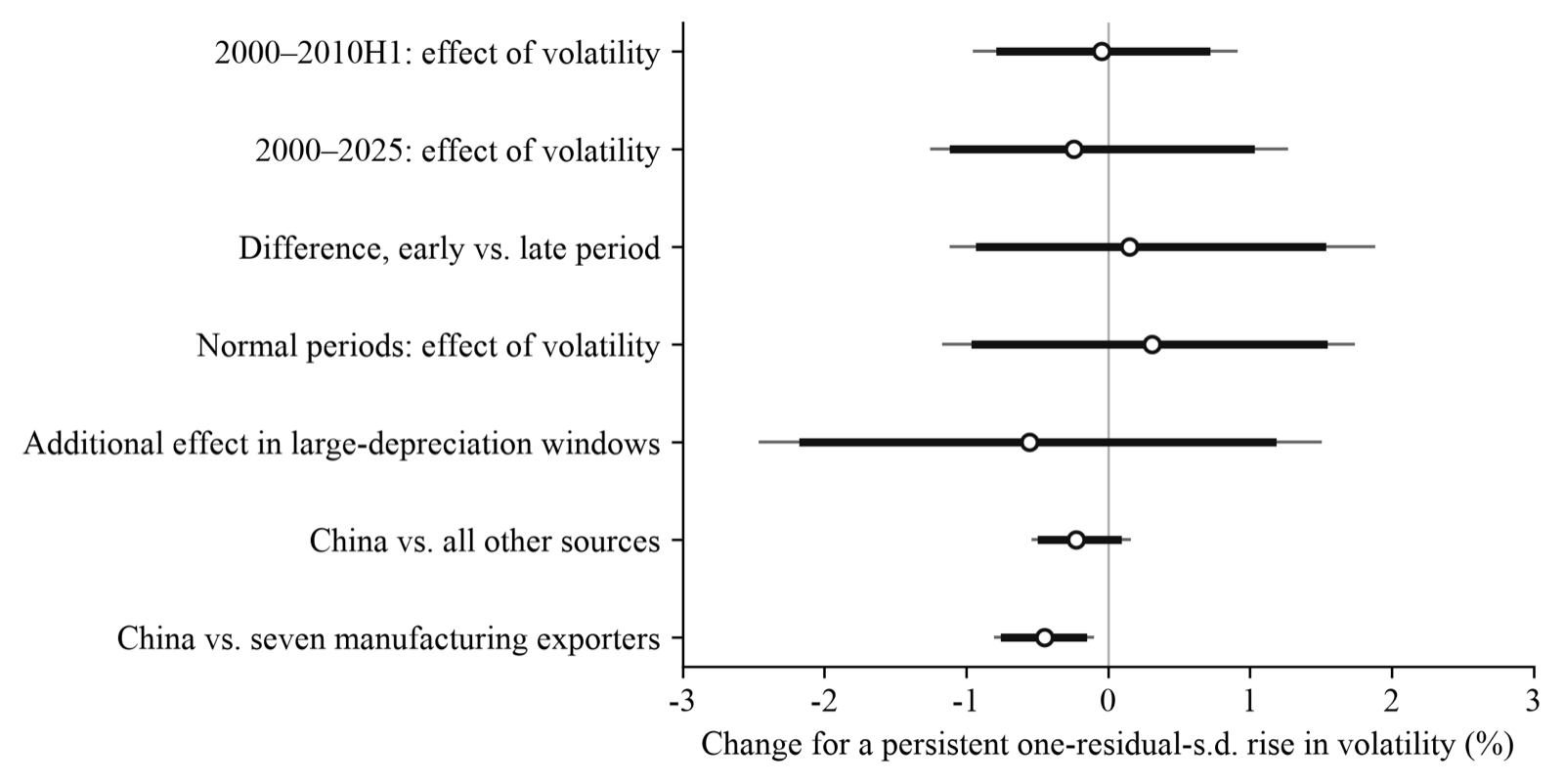
An insignificant result is informative only when it is clear what it rules out. Table 3 converts the coefficients into percentage changes in exports, and Figure 2 puts the estimates from all the main tests of this paper on the same scale. Measuring volatility by its residual standard deviation after removing the fixed effects, a persistent one-standard-deviation rise in partner-currency volatility changes China’s exports to that partner by −0.05% over January 2000–June 2010, with a 95% confidence set of [−0.94%, 0.90%]; by −0.23% from July 2010 onward, [−1.40%, 1.70%]; and by −0.24% in the full sample, [−1.24%, 1.26%]. For a larger change, namely a rise in volatility from the sample median to the 90th percentile, the full-sample confidence set is [−2.49%, 2.56%].
These intervals can be compared with existing estimates. Earlier firm-level studies measure volatility as the within-year standard deviation of monthly log changes in the exchange rate and report the change in exports for a rise of 0.01 in that measure. With about 21 trading days per month, this corresponds to a rise of about 0.218 percentage points in this paper’s standard deviation of daily returns (a monthly standard deviation of 0.01 is about 1/√21 ≈ 0.218 in daily terms, with daily returns in percentage points). On this scale, the full-sample effect in this paper is −0.30%, with a confidence set of [−1.57%, 1.60%]. The effects reported in the earlier literature, such as −0.04% in Tan et al. (2016, p. 23) and −0.51% in Wang et al. (2023, pp. 82–83), all fall within this interval, so this paper’s results do not contradict them; what this paper can rule out are effects about three times as large as the largest of these estimates (1.57/0.51 ≈ 3.1). Simulations with synthetic data show that the actual rejection rate of the wild score bootstrap at the 5% level is 4.5%–10.5%, so the confidence sets above may be somewhat too narrow, and some allowance should be made for this in interpretation.
The effective amount of information behind the intervals also needs to be stated. The full sample has 69 currencies, but the influence-weighted effective number of clusters is only 3.4, with the ruble and the Hong Kong dollar accounting for most of the influence; for the early sample it is 6.6. This is a common limitation of studies of bilateral exchange rate volatility: currencies that are pegged to the US dollar or that move closely together provide little independent variation. This paper therefore does not rely on CR1 standard errors, and Section 5 reports the results of dropping each currency in turn.
Table 3. Bounds on the effect: change in exports for a persistent rise in volatility (%)
| Sample | Residual s.d. | Rise of one residual s.d. | Rise from median to 90th percentile | Scale of earlier literature (ΔVOL = 0.218) | ||||
|---|---|---|---|---|---|---|---|---|
| Point estimate | 95% confidence set | 90% confidence set | Point estimate | 95% confidence set | Point estimate | 95% confidence set | ||
| January 2000–June 2010 | 0.139 | −0.05 | [−0.94, 0.90] | [−0.76, 0.69] | −0.12 | [−2.53, 2.47] | −0.07 | [−1.47, 1.42] |
| July 2010–December 2025 | 0.187 | −0.23 | [−1.40, 1.70] | [−1.21, 1.32] | −0.37 | [−2.29, 2.82] | −0.26 | [−1.62, 1.98] |
| Full sample | 0.172 | −0.24 | [−1.24, 1.26] | [−1.09, 1.01] | −0.48 | [−2.49, 2.56] | −0.30 | [−1.57, 1.60] |
| Full sample, normal periods (Equation 2) | 0.172 | 0.31 | [−1.16, 1.73] | [−0.94, 1.52] | 0.63 | [−2.33, 3.53] | 0.40 | [−1.47, 2.21] |
| Full sample, controlling for partner demand | 0.174 | 0.01 | [−1.00, 1.14] | [−0.82, 0.93] | 0.02 | [−1.99, 2.27] | 0.01 | [−1.26, 1.43] |
Note: The coefficient on V7 and its wild score bootstrap confidence set are converted into percentage changes in exports according to the size of the change in volatility. The residual standard deviation is the standard deviation of V7 after removing partner × year and year-month fixed effects; “rise from median to 90th percentile” is computed from the sample distribution of V7; the last two columns use the change in volatility of 0.218 commonly used in the earlier literature. The row “controlling for partner demand” corresponds to the specification in Table 4 that controls for the partner's imports from other sources.
5. Endogeneity and Robustness
5.1 Partner Demand
The main source of endogeneity in Equation (1) is the partner’s own demand shocks: currency turmoil often comes with a contraction of imports, and when the two occur together the volatility coefficient is biased toward negative values. This paper addresses this in two ways. First, it controls for the partner’s imports from other sources (current value and lags 1–6). With this control, the coefficient on V7 is 0.000 (bootstrap p = 0.99), and its confidence set converts to [−1.00%, 1.14%]; the cumulative coefficient on the demand terms is 0.41 and highly significant. Second, Equation (3) compares China with other suppliers within the same partner and month, so partner demand is fully absorbed by partner × year-month fixed effects; those results are reported in Section 6. Neither approach yields a significant effect. After directly controlling for partner demand, the point estimate moves from −0.017 (same subsample, without the control) to 0.000.
5.2 Sample and Specification
Table 4 reports the robustness checks listed in advance. For the full-sample estimates of Equation (1), dropping September 2008–December 2009, dropping January–February 2020, winsorizing V7 at the 1st and 99th percentiles, adding partner × calendar-month fixed effects, and setting volatility to missing when a month has fewer than 15 daily returns all yield coefficients between −0.021 and −0.009. Switching to OLS gives −0.024, and dropping currencies pegged to the US dollar or dropping Hong Kong SAR gives −0.036. For Equation (1), the smallest CV3 p-value is 0.25, and no specification is significant. For β in Equation (3), the coefficients range from −0.042 to +0.014 across specifications, and only one is significant: dropping currencies pegged to the US dollar (−0.042, CV3 p = 0.007), which Section 6.2 discusses. When the one-period lead of volatility is added as a placebo, its coefficient is −0.006 (CR1 p = 0.24).
When each currency is dropped in turn and the model is re-estimated, 68 of the 69 full-sample coefficients are negative, ranging from −0.036 (dropping the Hong Kong dollar) to +0.016 (dropping the ruble); for the early sample, the range is −0.022 to +0.008. The point estimate stays close to zero and slightly negative, and it does not depend on whether any single currency is included.
By subperiod, splitting the sample into four segments gives coefficients of −0.023, 0.002, 0.122, and −0.039, with CR1 p-values all above 0.12. The coefficients from 60-month rolling windows (Figure 3) turn to −0.113, −0.091, and −0.081 in the last three windows (2019–2023, 2020–2024, and 2021–2025), with CR1 p-values of 0.03–0.07; they are not significant under CV3 (0.11–0.31). The negative point estimates in recent years deserve attention, but the current evidence is not sufficient to call this a change.
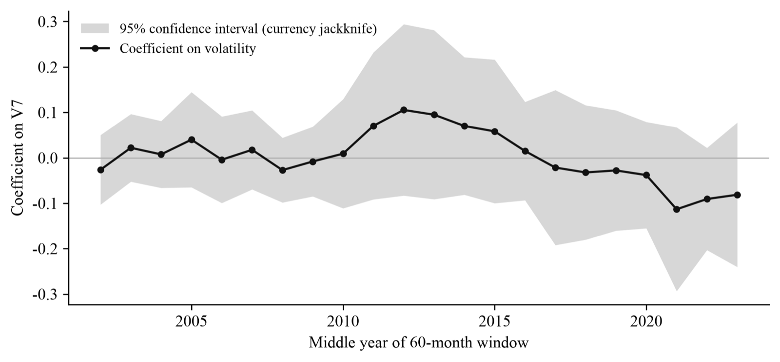
Table 4. Robustness checks
| Specification | Volatility V7 (Equation 1, full sample) | Additional effect in large-depreciation windows bc (Equation 2) | China relative to other sources β (Equation 3) |
|---|---|---|---|
| Baseline | −0.014 (0.033) [0.74] | −0.032 (0.053) [0.68] | −0.025 (0.016) [0.19] |
| Drop September 2008–December 2009 | −0.015 (0.034) [0.74] | −0.037 (0.062) [0.70] | −0.021 (0.017) [0.31] |
| Drop January–February 2020 | −0.011 (0.033) [0.80] | −0.038 (0.053) [0.63] | — |
| Winsorize V7 at the 1st and 99th percentiles | −0.012 (0.044) [0.82] | −0.073 (0.051) [0.21] | −0.017 (0.023) [0.52] |
| OLS (logs, zeros dropped) | −0.024 (0.016) [0.37] | 0.010 (0.034) [0.87] | −0.005 (0.017) [0.77] |
| Drop currencies pegged to the US dollar | −0.036 (0.023) [0.25] | −0.005 (0.044) [0.94] | −0.042 (0.013) [0.01] |
| Drop Hong Kong SAR | −0.036 (0.025) [0.28] | 0.000 (0.046) [1.00] | −0.029 (0.017) [0.17] |
| Add partner × calendar-month fixed effects | −0.021 (0.028) [0.57] | −0.046 (0.050) [0.55] | −0.024 (0.014) [0.13] |
| Volatility set to missing when the month has fewer than 15 daily returns | −0.009 (0.031) [0.82] | — | — |
| Control for partner imports from other sources (lags 0–6) | 0.000 (0.027) [0.99] | −0.001 (0.042) [0.98] | — |
| Exchange rate level also interacted with Crisis | — | −0.043 (0.042) [0.48] | — |
| Large-depreciation threshold set to 0.05 | — | −0.077 (0.046) [0.21] | — |
| Large-depreciation threshold set to 0.15 | — | −0.006 (0.051) [0.94] | — |
| Large-depreciation threshold set to 0.20 | — | 0.036 (0.052) [0.75] | — |
| Large-depreciation threshold set to V7 above the 99th percentile | — | −0.005 (0.073) [0.97] | — |
| All observations (including IMF imputations) | — | — | 0.014 (0.021) [0.62] |
Note: Each cell gives the coefficient, with the CR1 standard error clustered by currency in parentheses and the CV3 jackknife p-value in square brackets; “—” means that this specification was not run for that test. One-period-lead placebo: when the one-period lead of V7 is added to Equation (1), its coefficient is −0.006 (0.005), CR1 p = 0.241, CV3 p = 0.543; in the same regression, the coefficient on current V7 is −0.022 (0.036), CV3 p = 0.63.
6. Mechanisms and Heterogeneity
6.1 Normal Volatility and Large Depreciations: Hypothesis 3
Table 5 reports the results for Equation (2). The coefficient for normal periods, bn, is 0.018 (bootstrap p = 0.76); the additional effect within large-depreciation windows, bc, is −0.032 (p = 0.57); and the total effect within the windows is −0.014. Hypothesis 3 predicts that the effect is concentrated in periods of large depreciation, but the data show no difference between the two types of periods. The confidence set for bc converts to [−2.45%, 1.50%], wider than the [−1.16%, 1.73%] for normal periods, because large-depreciation partner–months make up only 2.2% of the sample and the effective number of clusters is 5.1. Changing the threshold from 0.10 to 0.05, 0.15, and 0.20 gives bc of −0.077, −0.006, and 0.036, respectively, none of them significant. At the level of total exports, this paper cannot determine whether currency crises hurt China’s exports more than normal volatility does.
Table 5. Normal volatility and large-depreciation windows
| Coefficient | CR1 s.e. | p-value: CR1 / CV3 / bootstrap | 95% confidence set (bootstrap) | Effect of a one-residual-s.d. rise (%) | |
|---|---|---|---|---|---|
| Normal periods bn | 0.018 | 0.043 | 0.670 / 0.726 / 0.758 | [−0.068, 0.100] | 0.31 [−1.16, 1.73] |
| Additional effect in large-depreciation windows bc | −0.032 | 0.053 | 0.542 / 0.678 / 0.570 | [−0.145, 0.087] | −0.56 [−2.45, 1.50] |
| Total within windows bn + bc | −0.014 | 0.040 | 0.718 / 0.824 / — | — | −0.25 |
| Crisis main effect | −0.013 | 0.054 | 0.814 / 0.878 / — | — | — |
Note: PPML estimates of Equation (2); fixed effects as in Equation (1). 27156 observations, 69 currencies; the effective numbers of clusters for bc and bn are 5.1 and 2.2, respectively. Effects are converted as in Table 3; “—” means not computed.
6.2 China Relative to Other Suppliers: Hypothesis 4
Panel A of Table 6 reports Equation (3). β is −0.025 (CR1 standard error 0.016), with a bootstrap p-value of 0.18, or 0.72 after the Holm correction; Hypothesis 4 is not supported. After conversion, a one-residual-standard-deviation rise in partner-currency volatility changes imports from China relative to imports from other sources by −0.22%, with a 95% confidence set of [−0.53%, 0.15%] and a 90% confidence set of [−0.47%, 0.07%]. This lies within the pre-specified equivalence bounds of ±2%. Estimated separately, the coefficient on volatility is −0.024 for imports from China and 0.003 for imports from other sources, and neither is significant.
One robustness check listed in advance departs from this conclusion. After dropping currencies pegged to the US dollar (Panel F of Table 6), β is −0.042, with a CV3 p-value of 0.007 and a bootstrap p-value of 0.017; converted to a one-residual-standard-deviation rise, the effect is −0.39%, with a 95% confidence set of [−0.70%, −0.10%]. Dropping only Hong Kong SAR gives β = −0.029 (CV3 p = 0.17), in the same direction but not significant. The result of the test of Hypothesis 4 is therefore sensitive to whether dollar-pegged currencies are included: among partners whose currencies are not pegged to the US dollar, imports from China fall slightly relative to imports from other suppliers when partner-currency volatility rises. This check is not in the family of tests corrected by Holm, the effect remains within the pre-specified ±2% equivalence bounds, and its direction matches that of Panel B below (relative to seven manufacturing exporters). This paper does not change its assessment of Hypothesis 4 on this basis, but treats the result, together with those in Section 6.3, as a lead to be tested.
As noted in Section 2, only if Hypothesis 4 fails and Hypothesis 1 holds does the effect work mainly on the importer side. Here both fail. At the bilateral level, no effect of partner-currency volatility can be detected either on China’s exports or on partners’ imports from other sources, and China’s position relative to other suppliers does not change as a result.
6.3 A Lead Still to Be Tested
Panels B–E of Table 6 are secondary analyses (Panels F–H are robustness checks on Panel A). Their results are not among the primary tests and are reported below only as leads. When the comparison group is changed from “all other sources” to seven manufacturing exporters, β is −0.050 (bootstrap p = 0.017). Split by period, β in normal periods is 0.004 and the additional term in large-depreciation windows is −0.059 (p = 0.043). Split by partner, β is 0.020 for advanced economies and −0.042 for emerging economies (p = 0.055). Taken together, relative to other manufacturing exporters, China’s exports fall more when the currencies of emerging economies depreciate sharply, by 0.4%–0.5% for a one-residual-standard-deviation rise.
This result cannot be taken as a conclusion, for four reasons. First, after the Holm correction, the smallest p-value among the four secondary analyses (comparison group, period, large depreciation, and emerging economies) is 0.066, and it is 0.083 if “using all observations” is also counted. Second, the decision on which analyses would also receive the bootstrap was made after seeing the CR1 and CV3 results. Third, with OLS (the log of the ratio of imports from China to imports from other sources), β is −0.005, and when the IMF-imputed observations are included it is +0.014; the PPML results are driven by a few large partners. Fourth, the result comes from monthly totals and cannot tell which products or which channels are involved. The direction it points to is clear: if partner-currency risk does affect China’s exports, the effect is more likely to appear during currency crises and in comparisons with similar suppliers than in everyday volatility and total exports. Testing this requires product-level import data and is left for future research.
Table 6. China relative to other suppliers
| Coefficient | CR1 s.e. | p-value: CR1 / CV3 / bootstrap | 95% confidence set (bootstrap) | Effect of a one-residual-s.d. rise (%) | Observations | |
|---|---|---|---|---|---|---|
| A. Relative to all other sources: β (primary test) | −0.025 | 0.016 | 0.122 / 0.187 / 0.181 | [−0.058, 0.016] | −0.22 [−0.53, 0.15] | 37318 |
| Separate estimation: imports from China | −0.024 | 0.019 | 0.196 / 0.280 / — | — | −0.22 | 18659 |
| Separate estimation: imports from other sources | 0.003 | 0.014 | 0.842 / 0.892 / — | — | 0.03 | 18659 |
| B. Relative to seven manufacturing exporters: β | −0.050 | 0.017 | 0.003 / 0.018 / 0.017 | [−0.087, −0.012] | −0.45 [−0.79, −0.11] | 37136 |
| C. Normal periods β | 0.004 | 0.022 | 0.871 / 0.891 / 0.875 | [−0.045, 0.051] | 0.03 [−0.41, 0.46] | 37318 |
| β × Crisis | −0.059 | 0.023 | 0.012 / 0.029 / 0.043 | [−0.116, −0.003] | −0.53 [−1.05, −0.03] | 37318 |
| D. Advanced-economy partners β | 0.020 | 0.027 | 0.463 / 0.571 / 0.493 | [−0.046, 0.075] | 0.18 [−0.42, 0.69] | 37318 |
| Emerging-economy partners β | −0.042 | 0.015 | 0.006 / 0.015 / 0.055 | [−0.076, 0.001] | −0.38 [−0.68, 0.01] | 37318 |
| β × EMDE | −0.062 | 0.028 | 0.029 / 0.077 / 0.077 | [−0.117, 0.008] | −0.56 [−1.06, 0.07] | 37318 |
| E. β × Early | 0.011 | 0.037 | 0.770 / 0.798 / 0.786 | [−0.068, 0.098] | 0.10 [−0.62, 0.89] | 37318 |
| F. Drop currencies pegged to the US dollar: β | −0.042 | 0.013 | 0.001 / 0.007 / 0.017 | [−0.075, −0.011] | −0.39 [−0.70, −0.10] | 34102 |
| G. All observations (including IMF imputations): β | 0.014 | 0.021 | 0.509 / 0.621 / — | — | 0.24 | 54174 |
| H. OLS, ln(from China / from other sources) | −0.005 | 0.017 | 0.760 / 0.768 / — | — | −0.05 | 18659 |
Note: Panel A is the primary test of Equation (3); the sample covers 79 partners and 64 currencies, the effective number of clusters is 8.1, and the 90% confidence set for the effect is [−0.47, 0.07]. The effective number of clusters for Panel B is 5.0. Panels B–E are secondary analyses; after the Holm correction, the bootstrap p-values of the four analyses B (comparison group), C (large depreciation), D (emerging economies), and E (period) are 0.066, 0.128, 0.153, and 0.786, respectively. Effects are converted as in Table 3; “—” means not computed.
6.4 Arbitrage-Driven Round-Tripping Trade
Export statistics may include round-tripping trade unrelated to real demand. Liu et al. (2023) find that when RMB interest rates exceed US dollar interest rates, mainland firms capture the interest rate differential by “exporting to Hong Kong and then re-importing,” and that this is more pronounced for goods with high value-to-weight ratios. Their re-import data end in 2017, and the differential was almost always positive within their sample. The 3-month moving average of the China–US 3-month interbank interest rate differential turned from positive to negative in September 2022 (the monthly value was already negative in August 2022) and stayed negative through the end of the sample period. This provides a test in the opposite direction. If arbitrage runs only one way, round-tripping should shrink with the differential; if funds instead use trade to stay abroad, round-tripping should expand with the size of the negative differential.
This paper tests these two possibilities with re-export data published by the Census and Statistics Department of the Hong Kong government. The dependent variable is the value of Hong Kong re-exports by HS four-digit heading, destination, and month (January 2012–December 2025, 1,098 headings, 30 destinations). The estimating equation is
RXp,d,t = exp[ β⁺ D⁺t zp CNd + β⁻ D⁻t zp CNd + αp,d + αp,t + αd,t ] εp,d,t (4)
where D⁺t and D⁻t are the absolute values of the differential when it is positive and when it is negative, respectively (3-month moving average); zp is the standardized log value-to-weight ratio (computed from the value and net weight of EU imports from outside the EU in 2011); and CNd indicates that the destination is the mainland. Heading × month fixed effects absorb changes in global supply and demand for each good, and destination × month fixed effects absorb overall changes in mainland demand and customs-clearance conditions. The specification, sample, inference method, and interpretation rules were written down by the author before the data were obtained (again, without registration on a third-party platform).
The results are in Table 7. β⁺ is 0.012 (standard error 0.027) and β⁻ is −0.001 (standard error 0.026), and neither is significant; without distinguishing sign, the coefficient is 0.008 (standard error 0.010). When the mainland is replaced in turn by each of the other 29 destinations, the mainland’s two coefficients rank 26th and 30th in absolute value. In addition, using “re-exports × origin × destination” data, with goods of mainland origin re-exported back to the mainland treated as a separate treated cell, the coefficients are likewise unremarkable in the permutation distribution of 198 placebo cells (permutation p-values of 0.97 and 0.46). Of the 11 robustness checks listed in advance, 9 do not change the conclusion. There are two exceptions. With a value-to-weight ratio × mainland × time trend added, β⁺ is 0.022 (p = 0.002), while β⁻ remains insignificant. When the differential is replaced by the realized carry return over the past 12 months, both coefficients are positive and significant; but this disappears after dropping Chapter 71 (gold and jewelry), and Hong Kong’s imports from the mainland show no corresponding change. This indicates that it comes from gold re-exports, not from widespread round-tripping arbitrage.
Two caveats are in order. First, the intervals are not narrow. When the differential falls from 0 to −3 percentage points, the 95% confidence interval for the relative change in mainland-bound re-exports of goods with a value-to-weight ratio one standard deviation higher is [−14.6%, +16.5%], and the OLS estimate weighting headings equally gives [−6.1%, +8.8%]; this paper cannot rule out smaller arbitrage effects. Second, public data cannot break down re-exports by origin and by product at the same time, and goods of mainland origin account for only 30% to 50% of re-exports to the mainland (49% in 2012 and about 32% since 2022), which would dilute any relationship that exists. Within these limits, this paper finds no evidence that the differential drives round-tripping of high-value goods, and no evidence in the opposite direction after the differential turned negative.
As a supplement, this paper also uses China’s reported monthly imports by chapter from UN Comtrade and compares re-imports with China as the origin against 9 other origins (January–September 2012 and January 2016–December 2024, 117 months in total; this test was added after seeing the Hong Kong results). β⁺ is 0.017 (standard error 0.028) and β⁻ is 0.060 (standard error 0.035, p = 0.085); after dropping Chapter 71, β⁻ falls to 0.028 (p = 0.47). Using only 2012–2017 and without distinguishing sign, the coefficient is 0.041 (standard error 0.035), in the same direction as in Liu et al. (2023) but not significant. Data aggregated by chapter have limited resolution, and these results do not change the conclusion above.
This section also yields a methodological result. Among the 29 placebo destinations unrelated to arbitrage, 14 (β⁺) and 12 (β⁻) have p-values below 0.05 with standard errors two-way clustered by heading and month. In panels of this “time-series shock × cross-sectional characteristic” type, clustered standard errors are clearly too small, and placebo distributions are a necessary complement.
Table 7. Interest rate differential and round-tripping trade via Hong Kong
| β⁺ (positive differential) | p-value | β⁻ (negative differential) | p-value | Observations | |
|---|---|---|---|---|---|
| A. Hong Kong re-exports, HS4 heading × destination × month | |||||
| Main specification | 0.012 (0.027) | 0.670 | −0.001 (0.026) | 0.976 | 2670676 |
| Add z × mainland × time trend | 0.022 (0.007) | 0.002 | −0.008 (0.039) | 0.835 | 2670676 |
| Drop February 2020–January 2023 | 0.023 (0.026) | 0.383 | 0.018 (0.020) | 0.381 | 2098199 |
| Drop Chapter 71 | 0.014 (0.026) | 0.584 | 0.013 (0.020) | 0.520 | 2611588 |
| Drop four headings including integrated circuits | 0.019 (0.027) | 0.468 | 0.008 (0.029) | 0.775 | 2650516 |
| OLS, ln(re-export value) | −0.013 (0.009) | 0.170 | 0.003 (0.012) | 0.779 | 1936214 |
| Differential replaced by realized carry return | 0.014 (0.006) | 0.026 | 0.013 (0.005) | 0.011 | 2670676 |
| Same, dropping Chapter 71 (post hoc) | −0.000 (0.002) | 0.795 | −0.009 (0.008) | 0.273 | 2611588 |
| B. Hong Kong imports from the mainland, HS4 heading × shipping origin × month | |||||
| Main specification | 0.014 (0.013) | 0.299 | 0.026 (0.019) | 0.179 | 2659278 |
| Differential replaced by realized carry return (post hoc) | −0.001 (0.003) | 0.829 | −0.008 (0.009) | 0.390 | 2659278 |
| C. China’s re-imports, HS chapter × origin × month (post hoc supplement) | |||||
| Main specification | 0.017 (0.028) | 0.549 | 0.060 (0.035) | 0.085 | 109502 |
| Drop Chapter 71 | 0.017 (0.031) | 0.573 | 0.028 (0.038) | 0.469 | 108332 |
Note: PPML estimates unless otherwise noted; standard errors two-way clustered by heading (chapter) and month are in parentheses. Panels A and B include heading × destination (shipping origin), heading × month, and destination (shipping origin) × month fixed effects, with the sample January 2012–December 2025; Panel C includes chapter × origin, chapter × month, and origin × month fixed effects, with the sample January–September 2012 and January 2016–December 2024. In the main specification of Panel A, the mainland's β⁺ and β⁻ rank 26th and 30th, respectively, in absolute value among the 30 destinations. The coefficients for the round-tripping cell (mainland origin, re-exported to the mainland) are 0.006 and 0.141, with permutation p-values among the 198 placebo cells of 0.97 and 0.46. In Panel C, using only 2012–2017 and without distinguishing sign, the coefficient is 0.041 (0.035), with a p-value of 0.238. Rows marked “post hoc” were added after seeing the results of the main specification.
7. Conclusions and Policy Implications
Using monthly data on China’s exports to 96 trading partners over 2000–2025, this paper tests the effect of partner-currency exchange rate volatility on China’s exports. None of the four hypotheses proposed in advance is supported. Higher partner-currency volatility does not significantly reduce China’s exports to that partner; this conclusion does not differ before and after 2010; there is no evidence that the effect is concentrated in periods of large partner-currency depreciation; and partners’ imports from China do not respond to the volatility of their currency significantly differently from their imports from other sources. The confidence sets confine the possible effect to a fairly small range: for a persistent rise in volatility of one residual standard deviation, the change in exports is no larger than about 1.3%, and the difference between China and other suppliers is no larger than about 0.5%. The exchange rate level, by contrast, has a significant effect: a 1% depreciation of the RMB against the partner currency raises exports to that partner by about 0.26% within half a year. Arbitrage-driven round-tripping trade in export statistics also shows no sign of moving with the interest rate differential.
The implications of these results have limits, and three points can be made with caution. First, for bilateral aggregates, the depressing effect of everyday partner-currency volatility on exports should not be overestimated. The shift of export markets toward emerging economies has not caused China’s aggregate exports to suffer noticeably from the normal volatility of these currencies. Second, changes in the exchange rate level deserve more attention than volatility: a sustained depreciation of a partner currency against the RMB has a measurable effect on China’s exports to that market. For exporting firms, managing the price and payment-collection risks that come with partner-currency depreciation matters more than hedging everyday volatility. Third, no conclusion can yet be drawn about the risks during currency crises. At the level of total exports, this paper finds no different effect in periods of large depreciation, but the effective information in this test is very small. Relative to similar suppliers, China’s exports to emerging economies fall more when their currencies depreciate sharply; if this lead is confirmed at the product level, it would point to export credit insurance, local-currency settlement, and hedging instruments for emerging-market currencies. The current evidence is not yet sufficient to support specific policy recommendations.
This paper has four limitations. First, the conclusions concern only the idiosyncratic volatility of partner currencies, not the common volatility of the RMB against the US dollar, and they have no direct implications for the exchange rate regime or exchange rate policy. Second, the data are bilateral monthly totals. A zero effect in the aggregate does not rule out responses of opposite sign or different size at the firm and product levels; the firm-level literature finds that financially constrained firms are more affected, and heterogeneity of this kind is averaged out in the aggregate. Third, the identifying variation is concentrated in a few currencies, and the wild score bootstrap confidence sets are somewhat too narrow in simulations, so the bounds in the text should be understood as approximate. Fourth, the test for arbitrage-driven round-tripping trade is constrained by public data: re-exports cannot be broken down by origin and by product at the same time, and re-imports are available only by chapter. The intervals are therefore wide, and smaller arbitrage effects cannot be ruled out.
Future research can proceed in two directions. One is to use “importing country × source country × product × month” data to compare different products and different suppliers during partner-currency crisis episodes, and to test whether products with long payment terms and a high degree of differentiation are more affected. The other is to use firm-level information on hedging and settlement currency to test the exporter-side channel directly.
References
Chinese-language entries marked [to be verified] have been seen only as citations in the reference lists of other works; the author has not yet checked the original publications. Volume, issue, and page details of the English-language entries have been checked against RePEc, Crossref, or the publisher’s pages. For the other entries, the notes in square brackets state what is still missing.
Cao Wei, Yan Fangrong, Bao Shuming. RMB exchange rate changes, the neighboring-country effect, and bilateral trade: An empirical study based on a spatial panel model of China and the countries along the “Belt and Road” [in Chinese][J]. Jinrong Yanjiu (Journal of Financial Research), 2016(9): 50-66.
Chen Ping, Xiong Xin. An empirical analysis of the effect of importing-country exchange rate volatility on China’s exports [in Chinese][J]. Guoji Jinrong Yanjiu (Studies of International Finance), 2002(6): 7-11. [to be verified]
Gu Yu, Gao Tiemei. An analysis of the effect of RMB exchange rate volatility on China’s imports and exports [in Chinese][J]. Shijie Jingji (The Journal of World Economy), 2007(10): 49-57. [to be verified]
Li Guangzhong, Voon L P. Real exchange rate misalignment, exchange rate volatility, and their effects on manufacturing exports: A panel data study, 1978–1998 [in Chinese][J]. Guanli Shijie (Management World), 2004(11): 22-28. [to be verified]
Lu Xiaodong, Liu Jingjun, Chen Zhijun. How do exporters hedge exchange rate risk? A value-chain integration perspective [in Chinese][J]. Guanli Shijie (Management World), 2019(5): 92-105+125. [to be verified]
Pan Hongyu. Exchange rate volatility and China’s exports to its major trading partners [in Chinese][J]. Shuliang Jingji Jishu Jingji Yanjiu (The Journal of Quantitative & Technical Economics), 2007(2): 73-81. [to be verified]
Peng Hongfeng, Liu Haiying. Theoretical measurement and analysis of the global-value-chain real effective exchange rate elasticity of bilateral exports [in Chinese][J]. Jinrong Yanjiu (Journal of Financial Research), 2021(2): 56-74.
Tan Xiaofen, Wang Yaqi, Lu Bing. Exchange rate volatility, financial marketization, and exports [in Chinese][J]. Jinrong Yanjiu (Journal of Financial Research), 2016(3): 15-30.
Wang Xue, Hu Weiming, Yang Haisheng. Exchange rate volatility and China’s bilateral export trade: Is there a third-country exchange rate effect? [in Chinese][J]. Jinrong Yanjiu (Journal of Financial Research), 2016(7): 1-16.
Wang Yaqi, Wang Yao, Zhang Liqing. The effect of exchange rate volatility on export stability: The role of intermediate goods imports [in Chinese][J]. Jinrong Yanjiu (Journal of Financial Research), 2023(1): 75-93.
Xu Yuan, Yu Yongze. The dampening role of financial development when exchange rate volatility shocks exports [in Chinese][J]. Jingji Kexue (Economic Science), 2016(6). [pages to be verified]
Abadie A, Athey S, Imbens G W, Wooldridge J M. When should you adjust standard errors for clustering?[J]. Quarterly Journal of Economics, 2023, 138(1): 1-35.
Bahmani-Oskooee M, Hegerty S. Exchange rate volatility and trade flows: A review article[J]. Journal of Economic Studies, 2007, 34(3): 211-255.
Boz E, Casas C, Georgiadis G, Gopinath G, Le Mezo H, Mehl A, Nguyen T. Patterns of invoicing currency in global trade: New evidence[J]. Journal of International Economics, 2022, 136: 103604.
Broda C, Romalis J. Identifying the relationship between trade and exchange rate volatility[M]//Ito T, Rose A K. Commodity Prices and Markets. Chicago: University of Chicago Press, 2011: 79-110.
Byrne J, Darby J, MacDonald R. US trade and exchange rate volatility: A real sectoral bilateral analysis[J]. Journal of Macroeconomics, 2008, 30(1): 238-259.
Canay I, Santos A, Shaikh A. The wild bootstrap with a “small” number of “large” clusters[J]. Review of Economics and Statistics, 2021, 103(2): 346-363.
Chit M, Rizov M, Willenbockel D. Exchange rate volatility and exports: New empirical evidence from the emerging East Asian economies[J]. The World Economy, 2010, 33(2): 239-263.
Clark P B. Uncertainty, exchange risk, and the level of international trade[J]. Western Economic Journal, 1973, 11(3): 302-313.
De Grauwe P. Exchange rate variability and the slowdown in growth of international trade[J]. IMF Staff Papers, 1988, 35(1): 63-84.
Ethier W. International trade and the forward exchange market[J]. American Economic Review, 1973, 63(3): 494-503.
Frankel J, Rose A. Currency crashes in emerging markets: An empirical treatment[J]. Journal of International Economics, 1996, 41(3-4): 351-366.
Gopinath G, Boz E, Casas C, Díez F J, Gourinchas P-O, Plagborg-Møller M. Dominant currency paradigm[J]. American Economic Review, 2020, 110(3): 677-719.
Hartman E, Hidalgo F D. An equivalence approach to balance and placebo tests[J]. American Journal of Political Science, 2018, 62(4): 1000-1013.
Héricourt J, Poncet S. Exchange rate volatility, financial constraints, and trade: Empirical evidence from Chinese firms[J]. The World Bank Economic Review, 2015, 29(3): 550-578.
Ilzetzki E, Reinhart C, Rogoff K. Exchange arrangements entering the twenty-first century: Which anchor will hold?[J]. Quarterly Journal of Economics, 2019, 134(2): 599-646.
Klein M, Shambaugh J. Fixed exchange rates and trade[J]. Journal of International Economics, 2006, 70(2): 359-383.
Kline P, Santos A. A score based approach to wild bootstrap inference[J]. Journal of Econometric Methods, 2012, 1(1): 23-41.
Li H, Ma H, Xu Y. How do exchange rate movements affect Chinese exports? — A firm-level investigation[J]. Journal of International Economics, 2015, 97(1): 148-161.
Liu X, Tang H, Wang Z, Wei S-J. Currency carry trade by trucks: The curious case of China’s massive imports from itself[J]. Review of Finance, 2023, 27(2): 469-493.
MacKinnon J G, Nielsen M Ø, Webb M D. Cluster-robust inference: A guide to empirical practice[J]. Journal of Econometrics, 2023, 232(2): 272-299.
MacKinnon J G, Webb M D. Wild bootstrap inference for wildly different cluster sizes[J]. Journal of Applied Econometrics, 2017, 32(2): 233-254.
McKenzie M. The impact of exchange rate volatility on international trade flows[J]. Journal of Economic Surveys, 1999, 13(1): 71-106.
Rainey C. Arguing for a negligible effect[J]. American Journal of Political Science, 2014, 58(4): 1083-1091.
Rose A. One money, one market: The effect of common currencies on trade[J]. Economic Policy, 2000, 15(30): 8-45.
Santos Silva J M C, Tenreyro S. The log of gravity[J]. Review of Economics and Statistics, 2006, 88(4): 641-658.
Tenreyro S. On the trade impact of nominal exchange rate volatility[J]. Journal of Development Economics, 2007, 82(2): 485-508.
Thorbecke W, Chen C, Salike N. The diminishing impact of exchange rates on China’s exports[J]. Japan and the World Economy, 2025, 76: 101329.
Wei S-J. Currency hedging and goods trade[J]. European Economic Review, 1999, 43(7): 1371-1394.